Three maps to examine the prevalence of intimate partner violence (IPV) in Cambodia

Developing choropleth maps with {ggplot2}, {sf}, and shapefiles

Overview

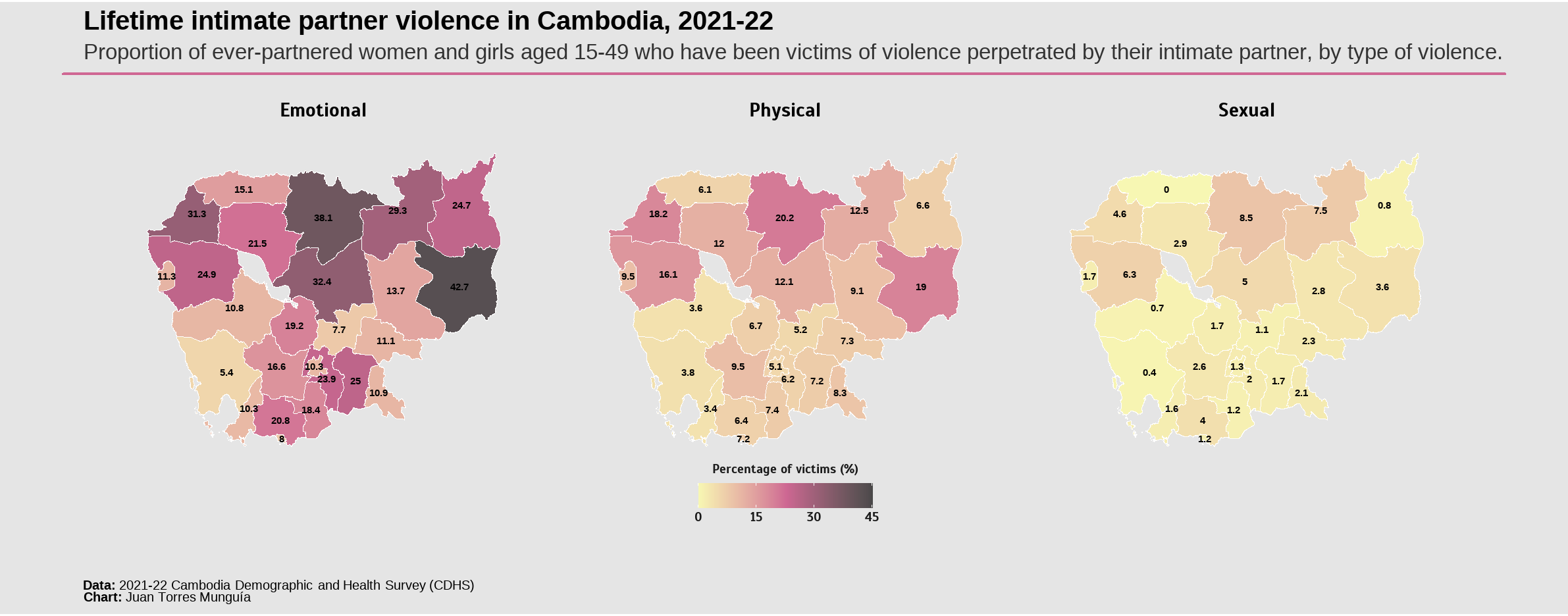
According to the 2021-22 Domestic Violence module of the Kingdom of Cambodia’s Demographic and Health Survey (CDHS), over 21% of Cambodian women aged 15–49 who have ever had a husband (or intimate partner), have experienced physical, sexual, economic, and/or emotional intimate partner violence in their lifetime. This figures varies significantly across the country, with some provinces reporting rates as high as 45% while others report rates as low as 6%.

A better understanding of the geographical distribution of intimate partner violence (IPV) in Cambodia can help policymakers and organizations to target their efforts more effectively. In this blog post, I will show how to create choropleth maps using R and shapefiles to visualize the prevalence of IPV in Cambodia at the provincial level. Additionally, I will use the {patchwork} package to combine these maps into the same graphic. The result will look like this:

About the data

Information comes from the document “Further Data Analysis Report. From the Cambodia Demographic and Health Survey 2021-2022”, available here. In particular, I will use Table A.1: Intimate-partner violence by background characteristics.

Set-up

First, we install and load the necessary R packages.

library(tidyverse) 
library(sf) # For handling shapefiles
library(readxl) # To read Excel files
library(kableExtra) # For data tables
library(ggplot2) 
library(ggtext) 
library(showtext) 
library(patchwork) # To combine multiple ggplots
library(colorspace) # For color palettes
library(grid) # To add lines and text elements to graphical objects

Loading data

I saved the information from Table A.1: Intimate-partner violence by background characteristics in the Excel file intimate-partner-violence-cambodia.xlsx.

ipv_cambodia <- read_excel("intimate-partner-violence-cambodia.xlsx")

This information looks like this:

ipv_cambodia |>
  kbl(
    caption = "Lifetime experience of specific acts of intimate partner physical violence committed by their current or most recent partner by provinces, Cambodia 2021-22"
    ) |>
  kable_paper("hover", full_width = F)

Lifetime experience of specific acts of intimate partner physical violence committed by their current or most recent partner by provinces, Cambodia 2021-22

Region	Emotional violence	Physical violence	Sexual violence	Physical or sexual	Physical or sexual or emotional	Number of women who ever had a husband/intimate partner
Banteay Meanchey	31.3	18.2	4.6	20.2	34.9	235
Battambang	24.9	16.1	6.3	19.8	30.4	378
Kampong Cham	7.7	5.2	1.1	5.8	11.5	352
Kampong Chhnang	19.2	6.7	1.7	6.7	19.2	213
Kampong Speu	16.6	9.5	2.6	10.1	19.1	362
Kampong Thom	32.4	12.1	5.0	14.4	35.1	242
Kampot	20.8	6.4	4.0	9.0	23.0	218
Kandal	23.9	6.2	2.0	6.5	23.9	423
Koh Kong	5.4	3.8	0.4	3.8	6.2	41
Kratie	13.7	9.1	2.8	10.2	15.9	138
Mondul Kiri	42.7	19.0	3.6	19.4	45.2	34
Phnom Penh	10.3	5.1	1.3	5.8	11.0	904
Preah Vihear	38.1	20.2	8.5	22.4	40.0	108
Prey Veng	25.0	7.2	1.7	8.6	26.3	366
Pursat	10.8	3.6	0.7	3.6	10.8	111
Ratanak Kiri	24.7	6.6	0.8	7.1	25.7	96
Siemreap	21.5	12.0	2.9	13.5	24.6	482
Preah Sihanouk	10.3	3.4	1.6	4.0	10.8	75
Stung Treng	29.3	12.5	7.5	16.3	31.5	66
Svay Rieng	10.9	8.3	2.1	8.8	13.6	217
Takeo	18.4	7.4	1.2	8.0	19.3	344
Otdar Meanchey	15.1	6.1	0.0	6.1	15.4	77
Kep	8.0	7.2	1.2	7.7	11.0	18
Pailin	11.3	9.5	1.7	9.5	14.2	29
Tboung Khmum	11.1	7.3	2.3	7.3	14.0	252

Now, we load geographical data of the administrative division of Cambodia. These data are obtained from the Humanitarian Data Exchange (HDX) initiative of the United Nations Office for the Coordination of Humanitarian Affairs (OCHA). The information comes as a shapefile .shp and is available here in a zip file named som_adm_ocha_20250108_AB_SHP.zip. I downloaded this file and located it in /khmadm_gov_20181004_ab_shp folder.

shp_cambodia <- read_sf("khmadm_gov_20181004_ab_shp/khm_admbnda_adm1_gov_20181004.shp")

Data wrangling

Next step is to combine the geographic information from the shapefile, shp_cambodia, with the data frame with the information on IPV, ipv_cambodia. To achieve this goal, we need to make sure that both datasets have a common variable to merge them. In this case, we will use the province name ADM1_EN in the shapefile and Region in the data frame. Then, I compare if the names of the provinces in both datasets match:

setdiff(shp_cambodia$ADM1_EN, ipv_cambodia$Region)

[1] "Oddar Meanchey"

The output indicates that there is one discrepancy. In shp_cambodia, the name of the province “Oddar Meanchey” corresponds to “Otdar Meanchey” in ipv_cambodia. I will rename this province in the shapefile to match the name in the data from the official report.

shp_cambodia <- shp_cambodia |>
  mutate(ADM1_EN = case_when(
    ADM1_EN == "Oddar Meanchey" ~ "Otdar Meanchey",
    TRUE ~ ADM1_EN
  ))

After this modification, I join both datasets using a left join to keep all the provinces in the shapefile and add the corresponding IPV values from the data frame:

shp_cambodia <- shp_cambodia |>
  left_join(ipv_cambodia, by = c("ADM1_EN" = "Region"))

Creating the map

My idea is to develop three maps, each representing one type of violence against women and girls: emotional, physical, and sexual. I will first create the map corresponding to emotional violence.

# More font alternatives can be found here https://fonts.google.com/
font_add_google("Scada", "Scada") 

showtext_auto()

map_ipv_emotional_cambodia <- ggplot() +
  geom_sf(
    data = shp_cambodia, 
    aes(fill = `Emotional violence`), 
    color = "white", # Color of the province borders
    linewidth = 0.5
  ) +
  geom_sf_text(
    data = shp_cambodia,
    aes(label = `Emotional violence`),
    check_overlap = TRUE, # To avoid overlaping text in the plot
    size = 4, 
    color = "black",
    fontface = "bold"
  ) +
  scale_fill_gradient2(
    low = "#FFFE9EB3",
    mid = "#C53270B3",
    high = "#040404B3",
    midpoint = 22.5,
    limits = c(0, 45),
    breaks = c(0, 15, 30, 45),
    labels = c("0", "15", "30", "45")
  ) +
  labs(
    title = "Emotional", # Title of this subplot
    subtitle = "",
    caption = "",
    x = "",
    y = "",
    fill = "Percentage of victims (%)" # Title of the legend
  ) +
  theme_minimal(
    base_family = "Scada"
  ) +
  theme(
    plot.margin = margin(0, 40, 0, 40),
    
    plot.background = element_blank(), # No color in the background
    plot.title = element_text(
      color = "black",
      face = "bold",
      size = 22,
      hjust = 0.5,
      margin = margin(5, 0, 5, 0)
    )
  )

Now, I replicate the same format for physical and sexual violence.

map_ipv_physical_cambodia <- ggplot() +
  geom_sf(
    data = shp_cambodia, 
    aes(fill = `Physical violence`), 
    color = "white", 
    linewidth = 0.5
  ) +
  geom_sf_text(
    data = shp_cambodia,
    aes(label = `Physical violence`),
    check_overlap = TRUE,
    size = 4, 
    color = "black",
    fontface = "bold"
  ) +
  scale_fill_gradient2(
    low = "#FFFE9EB3",
    mid = "#C53270B3",
    high = "#040404B3",
    midpoint = 22.5,
    limits = c(0, 45)
  ) +
  labs(
    title = "Physical",
    subtitle = "",
    caption = "",
    x = "",
    y = "",
    fill = ""
  ) + 
  guides(fill = "none") +
  theme_minimal(
    base_family = "Scada"
  ) +
  theme(
    plot.margin = margin(0, 40, 0, 40),
    
    plot.background = element_blank(),
    plot.title = element_text(
      color = "black",
      face = "bold",
      size = 22,
      hjust = 0.5,
      margin = margin(5, 0, 5, 0)
    )
  )

map_ipv_sexual_cambodia <- ggplot() +
  geom_sf(
    data = shp_cambodia, 
    aes(fill = `Sexual violence`), 
    color = "white", 
    linewidth = 0.5
  ) +
  geom_sf_text(
    data = shp_cambodia,
    aes(label = `Sexual violence`),
    check_overlap = TRUE,
    size = 4, 
    color = "black",
    fontface = "bold"
  ) +
  scale_fill_gradient2(
    low = "#FFFE9EB3",
    mid = "#C53270B3",
    high = "#040404B3",
    midpoint = 22.5,
    limits = c(0, 45)
  ) +
  labs(
    title = "Sexual",
    subtitle = "",
    caption = "",
    x = "",
    y = "",
    fill = ""
  ) + 
  guides(fill = "none") +
  theme_minimal(
    base_family = "Scada"
  ) +
  theme(
    plot.margin = margin(0, 40, 0, 40),
    
    plot.background = element_blank(),
    plot.title = element_text(
      color = "black",
      face = "bold",
      size = 22,
      hjust = 0.5,
      margin = margin(5, 0, 5, 0)
    )
  )

Now, using {patchwork} package, I combine the three plots into one single representation. I also use plot_annotation() function to add a title, subtitle, and caption to the overall design.

# Design display two rows, one with the three maps, and the second one only with the common guide
map_ipv_cambodia <- (map_ipv_emotional_cambodia + map_ipv_physical_cambodia + map_ipv_sexual_cambodia) / guide_area() + 
  # Custom title, subtitle, and caption
  plot_annotation(
    title = "Intimate partner violence in Cambodia, 2021-22",
    subtitle = "Proportion of ever-partnered women and girls aged 15-49 who have been victims of violence perpetrated by their intimate partner, by type of violence.",
    caption = "**Data:** 2021-22 Cambodia Demographic and Health Survey (CDHS) <br> **Chart:** Juan Torres Munguía",
    theme = theme(
      # Title settings
      plot.title.position = "plot", 
      plot.title = element_text(
        color = "black",
        face = "bold",
        size = 30,
        hjust = 0,
        margin = margin(5, 0, 5, 50)
      ),
      
      plot.subtitle = element_text(
        color = "grey20",
        size = 25,
        hjust = 0,
        margin = margin(5, 0, 40, 50)
        ),
        
        # Caption settings
        # I use element_markdown() because the caption has markdown text
        plot.caption = element_markdown(
          color = "black",
          size = 15,
          hjust = 0,
          margin = margin(80, 0, 5, 50)
        )
  )) +

  plot_layout(guides = "collect",
              heights = unit(c(13, 1),
               c('cm', 'cm'))
              ) + 
  theme_minimal(
    base_family = "Scada"
  ) &
  # Custom theme settings
  theme(
    legend.background = element_blank(),
    legend.position = "bottom",
    legend.title = element_text(
      margin = margin(5, 0, 10, 0),
      face = "bold",
      color = "grey10",
      size = 14,
      hjust = 0.5
    ),
    legend.title.position = "top",
    legend.text = element_text(
      margin = margin(5, 5, 5, 5), 
      face = "bold",
      color = "grey10",
      size = 14
    ),
    legend.key.width = unit(1.4, "cm"),
    legend.key.height = unit(1, "cm"),
    legend.direction = "horizontal",

    plot.background = element_rect(
      color = "#E5E5E5",
      fill = "#E5E5E5"),
    # Axis settings
    axis.title = element_blank(),
    axis.line = element_blank(),
    axis.text = element_blank(),
    axis.ticks = element_blank(),
    panel.grid = element_blank()
    
  )

Finally, I use grid.lines() from {grid} package to add a horizontal line after the subtitle.

map_ipv_cambodia

grid.lines(
  x = c(0.04, 0.96), # Values should be between 0 and 1
  y = 0.88, # Value should be between 0 and 1
  gp = gpar(col = "#C53270B3", 
            lwd = 4)
)